Simplified spring model for coupling two bodies

[Nobody-86]

Hello everyone,

I would like to couple two bodies together via a spring element. In reality, the two bodies are in contact with each other (sometimes also via a third body), but a contact calculation is too time-consuming. Instead, I would prefer to reduce the nodes in contact to one node per side via a *DISTRIBUTING COUPLING and define a SPRINGA spring element between the two remaining nodes. This is how I know it from other FE programs (ANSYS). Furthermore, the stiffness is not isotropic, but depends on the spatial directions. Fortunately, it is always Cartesian.

However, there are three difficulties.

1. According to the help for *DISTRIBUTING COUPLING, the reference node may only be used for the DCOUP3D element and only for boundary conditions. It should not be linked to other elements.
2. The reference nodes are usually concentric. For the SPRINGA spring element, the nodes must not be concentric.
3. The SPRINGA spring element has only one stiffness, and the direction results from the relative positions of the coupling nodes. The nodes could be rotated with the *TRANSFORM command into the coordinate system in which I know the stiffnesses in X, Y & Z, but I don’t know how to define the spring element so that it has different stiffnesses in X, Y & Z.

All three problems look impossible for me to solve, so I suspect that I have overlooked something fundamental. Maybe my approach is wrong, it’s just the one I know from ANSYS. Maybe such a connection is modeled completely differently in Calculix / Abaqus. It would be super nice if someone here could give me a modeling approach.

[Calc_em]

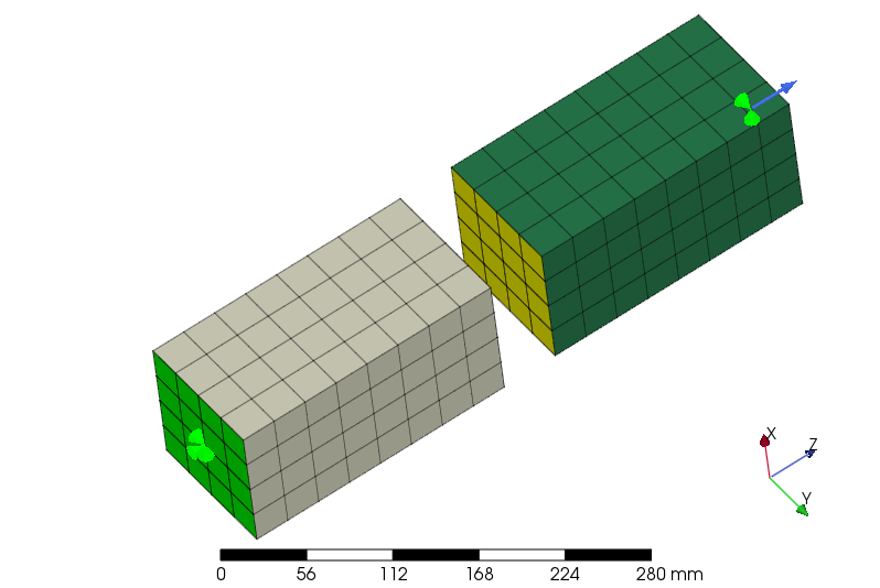
You could use 3 SPRING2 elements and attach them to rigid body reference nodes. Like this:

*Node
1, 0.00000000E+000, 0.00000000E+000, 0.00000000E+000
2, 0.00000000E+000, 0.00000000E+000, 1.00000000E+001
3, 0.00000000E+000, 1.00000000E+001, 0.00000000E+000
4, 0.00000000E+000, 1.00000000E+001, 1.00000000E+001
5, 1.00000000E+001, 0.00000000E+000, 0.00000000E+000
6, 1.00000000E+001, 0.00000000E+000, 1.00000000E+001
7, 1.00000000E+001, 1.00000000E+001, 0.00000000E+000
8, 1.00000000E+001, 1.00000000E+001, 1.00000000E+001
9, 0.00000000E+000, 0.00000000E+000, 5.00000000E+000
10, 0.00000000E+000, 5.00000000E+000, 0.00000000E+000
11, 0.00000000E+000, 1.00000000E+001, 5.00000000E+000
12, 0.00000000E+000, 5.00000000E+000, 1.00000000E+001
13, 1.00000000E+001, 0.00000000E+000, 5.00000000E+000
14, 1.00000000E+001, 5.00000000E+000, 0.00000000E+000
15, 1.00000000E+001, 1.00000000E+001, 5.00000000E+000
16, 1.00000000E+001, 5.00000000E+000, 1.00000000E+001
17, 5.00000000E+000, 0.00000000E+000, 0.00000000E+000
18, 5.00000000E+000, 0.00000000E+000, 1.00000000E+001
19, 5.00000000E+000, 1.00000000E+001, 0.00000000E+000
20, 5.00000000E+000, 1.00000000E+001, 1.00000000E+001
21, 0.00000000E+000, 5.00000000E+000, 5.00000000E+000
22, 1.00000000E+001, 5.00000000E+000, 5.00000000E+000
23, 5.00000000E+000, 0.00000000E+000, 5.00000000E+000
24, 5.00000000E+000, 1.00000000E+001, 5.00000000E+000
25, 5.00000000E+000, 5.00000000E+000, 0.00000000E+000
26, 5.00000000E+000, 5.00000000E+000, 1.00000000E+001
27, 5.00000000E+000, 5.00000000E+000, 5.00000000E+000
28, 1.50000000E+001, 0.00000000E+000, 0.00000000E+000
29, 1.50000000E+001, 0.00000000E+000, 1.00000000E+001
30, 1.50000000E+001, 1.00000000E+001, 0.00000000E+000
31, 1.50000000E+001, 1.00000000E+001, 1.00000000E+001
32, 2.50000000E+001, 0.00000000E+000, 0.00000000E+000
33, 2.50000000E+001, 0.00000000E+000, 1.00000000E+001
34, 2.50000000E+001, 1.00000000E+001, 0.00000000E+000
35, 2.50000000E+001, 1.00000000E+001, 1.00000000E+001
36, 1.50000000E+001, 0.00000000E+000, 5.00000000E+000
37, 1.50000000E+001, 5.00000000E+000, 0.00000000E+000
38, 1.50000000E+001, 1.00000000E+001, 5.00000000E+000
39, 1.50000000E+001, 5.00000000E+000, 1.00000000E+001
40, 2.50000000E+001, 0.00000000E+000, 5.00000000E+000
41, 2.50000000E+001, 5.00000000E+000, 0.00000000E+000
42, 2.50000000E+001, 1.00000000E+001, 5.00000000E+000
43, 2.50000000E+001, 5.00000000E+000, 1.00000000E+001
44, 2.00000000E+001, 0.00000000E+000, 0.00000000E+000
45, 2.00000000E+001, 0.00000000E+000, 1.00000000E+001
46, 2.00000000E+001, 1.00000000E+001, 0.00000000E+000
47, 2.00000000E+001, 1.00000000E+001, 1.00000000E+001
48, 1.50000000E+001, 5.00000000E+000, 5.00000000E+000
49, 2.50000000E+001, 5.00000000E+000, 5.00000000E+000
50, 2.00000000E+001, 0.00000000E+000, 5.00000000E+000
51, 2.00000000E+001, 1.00000000E+001, 5.00000000E+000
52, 2.00000000E+001, 5.00000000E+000, 0.00000000E+000
53, 2.00000000E+001, 5.00000000E+000, 1.00000000E+001
54, 2.00000000E+001, 5.00000000E+000, 5.00000000E+000
55, 1.00000000E+001, 5.00000000E+000, 5.00000000E+000
56, 1.00000000E+001, 5.00000000E+000, 5.00000000E+000
57, 1.50000000E+001, 5.00000000E+000, 5.00000000E+000
58, 1.50000000E+001, 5.00000000E+000, 5.00000000E+000
*Element, Type=C3D8, Elset=Solid_part-1
1, 21, 9, 1, 10, 27, 23, 17, 25
2, 27, 23, 17, 25, 22, 13, 5, 14
3, 11, 21, 10, 3, 24, 27, 25, 19
4, 24, 27, 25, 19, 15, 22, 14, 7
5, 12, 2, 9, 21, 26, 18, 23, 27
6, 26, 18, 23, 27, 16, 6, 13, 22
7, 4, 12, 21, 11, 20, 26, 27, 24
8, 20, 26, 27, 24, 8, 16, 22, 15
*Element, Type=C3D8, Elset=Solid_part-2
9, 48, 36, 28, 37, 54, 50, 44, 52
10, 54, 50, 44, 52, 49, 40, 32, 41
11, 38, 48, 37, 30, 51, 54, 52, 46
12, 51, 54, 52, 46, 42, 49, 41, 34
13, 39, 29, 36, 48, 53, 45, 50, 54
14, 53, 45, 50, 54, 43, 33, 40, 49
15, 31, 39, 48, 38, 47, 53, 54, 51
16, 47, 53, 54, 51, 35, 43, 49, 42
*ELEMENT, TYPE=SPRING2, ELSET=SPRING_X
100,55,57
*ELEMENT, TYPE=SPRING2, ELSET=SPRING_Y
200,55,57
*ELEMENT, TYPE=SPRING2, ELSET=SPRING_Z
300,55,57
*SPRING, ELSET=SPRING_X
1,1
100.
*SPRING, ELSET=SPRING_Y
2,2
100.
*SPRING, ELSET=SPRING_Z
3,3
100.
*Nset, Nset=Internal_Selection-1_Rigid_Body-1
5, 6, 7, 8, 13, 14, 15, 16, 22
*Nset, Nset=Internal_Selection-1_Rigid_Body-2
28, 29, 30, 31, 36, 37, 38, 39, 48
*Nset, Nset=Internal_Selection-1_Fixed-1
1, 2, 3, 4, 9, 10, 11, 12, 21
*Nset, Nset=Internal_Selection-1_Displacement_Rotation-1
32, 33, 34, 35, 40, 41, 42, 43, 49
*Nset, Nset=Reference_Point-1_ref_55
55
*Nset, Nset=Reference_Point-1_rot_56
56
*Nset, Nset=Reference_Point-2_ref_57
57
*Nset, Nset=Reference_Point-2_rot_58
58
*Elset, Elset=Internal_Selection-1_Solid_Section-1
Solid_part-1, 
Solid_part-2
*Material, Name=S235
*Elastic
210000, 0.28
*Solid section, Elset=Internal_Selection-1_Solid_Section-1, Material=S235
*Rigid body, Nset=Internal_Selection-1_Rigid_Body-1, Ref node=55, Rot node=56
*Rigid body, Nset=Internal_Selection-1_Rigid_Body-2, Ref node=57, Rot node=58
*Step
*Static
*Boundary
Internal_Selection-1_Fixed-1, 1, 6, 0
*Boundary
Internal_Selection-1_Displacement_Rotation-1, 1, 1, 0
Internal_Selection-1_Displacement_Rotation-1, 2, 2, 0
Internal_Selection-1_Displacement_Rotation-1, 3, 3, 1
*Node file
RF, U
*El file
S, E, NOE
*End step

[Nobody-86]

Great! That looks very much like what I need. I’ll try to adapt the example to my usecase. Many thanks!

[lucas_bueno]

@Nobody-86

It should not be linked to other elements.

I verified this does not apply to mass elements, even if the documentation states otherwise. Maybe for springs, it can work as well.

[vicmw]

You can use contact with the TIED parameter which works with linear analysis so it’s fast, and connects the faces with linear springs.

Yea *DISTRIBUTING COUPLING and *DISTRIBUTING have no special powers in CCX. It’s just an alternative way of applying loads that you could also do using *CLOAD and correct choice of values.

[xyont]

@lucas_bueno

Maybe for springs, it can work as well.

yes it seems possible to connect by equation constraint. Distributing coupling also can be work for another case of connector, but limited to translation DOF’s only.

depend on analysis cases, *Coupling type *Distributing will work for bc’s type force, it will similar to RBE3. can not be used as connector of element (e.g beam and shell). *Rigid body constraint also the same, except in over-stiffening the model. it may similar to RBE2

*Distributing coupling with Dcoup3d element also will gave similar with RBE3 for cases a connector between element, but limited to translation only. not has any rotational transmitted.

[xyont]

@vicmw

You can use contact with the TIED parameter which works with linear analysis so it’s fast, and connects the faces with linear springs.

yes, it use linear spring as in contact algorithm. However, the quantity or sum of spring value is hard to know since the patch nodes or integration point of element face is generated automatically by the solver. Also, not to depending on surface areas connected.

it seems these approach only appropriates for total force transmitted (full, partially or separates) not the sum of spring stiffness in connection itself.

[vicmw]

I think the total spring stiffness for TIED contact is accurate (contact stiffness * area). I’ve tested that at least on simple meshes.

[xyont]

interesting when you have been tested. Previously, i was thinking also since the units are in force per cubic volume and multiplied by areas lead to stiffness in force per length. But, another section describes its individual stiffness with no relation with surface tributary areas, the highest value means hard contact.

[vicmw]

Here’s a test:
Contact stiffness = 300
Area = 4
Total stiffness = 300 * 4 = 1200
Force = 1200
Displacement = 1200 / 1200 = 1 agrees with solution.

** Generated by Mecway 25
*NODE
1,10,0,1
2,10,1,1
3,10,2,1
4,10,1,1
5,12,1.5,2
6,10,1.5,2
7,10,0.5,2
8,12,1,0
9,11,2,2
10,10,2,0
11,11,0,0
12,12,0.5,0
13,11,1,0
14,10,1,2
15,12,0,1
16,12,1,2
17,12,2,2
18,12,0,2
19,12,1,2
20,10,2,2
21,12,1,1
22,11,0,2
23,12,0.5,2
24,11,1,2
25,11,1,0
26,12,1.5,0
27,11,2,0
28,12,1,1
29,10,1,0
30,10,0,0
31,10,1,0
32,12,1,0
33,12,2,0
34,10,0,2
35,10,1,2
36,12,2,1
37,10,1.5,0
38,12,0,0
39,10,0.5,0
40,11,1,2
*ELEMENT,TYPE=C3D20
1,29,32,33,10,14,16,17,20,25,26,27,37,40,5,9,
6,2,28,36,3
2,30,38,8,31,34,18,19,35,11,12,13,39,22,23,24,
7,1,15,21,4
*ELSET,ELSET=Default
1
2
*SURFACE,NAME=contact_faces(2)
1,S3
*SURFACE,NAME=contact_faces
2,S5
*MATERIAL,NAME=Material
*ELASTIC,TYPE=ISOTROPIC
50000000000,0
*SOLID SECTION,ELSET=Default,MATERIAL=Material
*BOUNDARY
1,1,,0
1,2,,0
1,3,,0
11,1,,0
11,2,,0
11,3,,0
15,1,,0
15,2,,0
15,3,,0
18,1,,0
18,2,,0
18,3,,0
22,1,,0
22,2,,0
22,3,,0
30,1,,0
30,2,,0
30,3,,0
34,1,,0
34,2,,0
34,3,,0
38,1,,0
38,2,,0
38,3,,0
*CONTACT PAIR,INTERACTION=SI_1,TYPE=SURFACE TO SURFACE,ADJUST=34.64101615138
contact_faces(2),contact_faces
*SURFACE INTERACTION,NAME=SI_1
*SURFACE BEHAVIOR,PRESSURE-OVERCLOSURE=TIED
300
*FRICTION
1,300
*STEP
*STATIC
*CLOAD
33,2,-100
10,2,-100
17,2,-100
20,2,-100
27,2,400
36,2,400
3,2,400
9,2,400
*NODE FILE,GLOBAL=YES,CONTACT ELEMENTS
U,RF
*EL FILE
S,NOE,E,ENER
*END STEP

[xyont]

it seems to be right, K value of slope of the pressure-overclossure curve is individual stiffness which have no relation with surface areas. As shown in deflection result is way off compared to another software and simple analytical.

below several sreenshot of my simple test,

*edited,
may i correcting, previously i miss dividing the stiffness with surface area connected, K value should be 42N/mm3 instead then result become identical. Thanks for introducing some example problems.

as in early states, i have no doubt about K value of pressure-overclosure is related to global stiffness and force transmitted. Only quantifying the sum of stiffness at surface area is questionable.

[Disla]

@xyont

simple analytical

Seem “simple analytical” need more investigation.
Also sudden new uniform displacent can’t be explained. Result similar to imposed displacement curious match results.

[vicmw]

I’m confused. Looks like your updated result (bottom picture) agrees with your hand calc but you say the sum of the stiffness is questionable?

[xyont]

i mean previously did not know how quantifying, it’s clear then.

[Disla]

According to simply hand calculation three elements with different sections were loaded with 10KN. Modeling that agrees perfectly.

Tie contact stiffness should be defined on a surface area of 10mmx10mm.
Contact was unfortunately defined on the whole section. I say that because model shows a 100mmx100mm brick meshed 4x4 which gives squares areas of 25x25. Impossible contact was properly defined.
Solid displacements shown right on the picture , but none of those elements are of interest In this topic but the gap generated in the contact.
Good to erase picture and I also suggest correct hand calculation (A2=10mmx10mm) to match model.

[Nobody-86]

Thanks again to everyone for all the suggestions. I’ve done a lot of tinkering in the meantime and so far everything works as I imagined for simple models.

With more complex models, the results sometimes seem implausible to me. I would like to check two things for debugging, but I don’t know how.

1. I have rotated some nodes to other coordinate systems using the *TRANSFORM command. Can I somehow display the local alignment of the nodes visually? So that I can check whether they are all correctly aligned?

2. Is there a way to output or visually display the force in the SPRING2 elements?

[JuanP74]

@Nobody-86

I have rotated some nodes to other coordinate systems using the *TRANSFORM command. Can I somehow display the local alignment of the nodes visually?

not sure what you mean but I think there is a misunderstanding here:

*TRANSFORM,NSET=No1,TYPE=R
0.,1.,0.,0.,0.,1.

assigns a new rectangular coordinate system to the nodes belonging to (node)
set No1. The x- and the y-axes in the local system are the y- and z-axes in the
global system.
Example files: segment1, segment2, segmentf, segmentm.

transform WILL NOT move any node, but will change the coordinate system in which boundary conditions are applied

[Nobody-86]

I didn’t want to move the node, I wanted to rotate it. I drew a sketch to illustrate what I had in mind. On the left in the picture, I move the dark blue dot vertically upwards to the light blue dot. The distance traveled from the node is, for example, 0 mm in the X direction and 1 mm in the Y direction.
However, if the node is rotated (right image), e.g. by 45°, the displacement in the local coordinate system of the node is 0.71 mm in the X direction and also in the Y direction.

I wanted to orient the nodes so that they are normal to a surface and coupled with the SPRING2 element. The aim was to ensure that forces are only absorbed and transmitted in this direction.

If the node were connected to another (fixed) node with a SPRING2 element and the spring element had a stiffness of 100 N/mm in Y direction, a force of 100N would result in the left image. In the right image with the rotated node, it would be just 71kN.

[Calc_em]

Technically, the node is not rotated when applying *TRANSFORM to it. This keyword only assigns a local coordinate system to that node and all BCs and nodal forces are acting in that system from now on. So yeah, you can use this to make BC definitions more convenient.

[Nobody-86]

I re-read the manual and realized that I had really misunderstood something here. I was convinced that *TRANSFORM applies not only to boundary conditions, but also to the orientation of SPRING1/2 elements. But now I have seen that there is an extra keyword for this: *ORIENTATION, as well as the corresponding parameter in the *SPRING command.

I’m currently testing whether I can achieve what I want with it. The second part of my question would also be important so that I can debug better: Is there a way to output and visualize the force in SPRING2 elements?