Acceleration output for dynamic calculations

Hello!

I’ve created a PR that adds the A option for *NODE FILE to output the accelerations [ACCE] to the .frd file.

As a beginner CalculiX user, I would appreciate some help constructing a simple verification example. I’ve used pendel.inp to test the functionality, but I am uncertain about the correctness of the output.

First, thanks for your work. Hopefully, we are in time to include it in the next release.

My proposal is a rotating cube like the one attached.

As each node describes a circle and travels at constant angular velocity there is only centripetal acceleration (ac = ω²r)

Angular velocity w is set to 1 revolution / second = 2*pi radians/s

r=distance for base middle nodes to the z axis=1m

Midside node number 10 expected results:

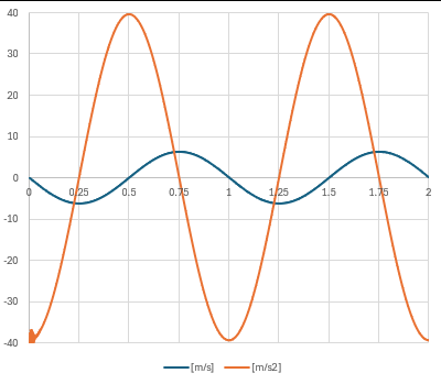
Magnitude v=w*r=sqrt(vx^2+vy^2)=6.28 m/s

Magnitude ac=sqrt(ax^2+ay^2)=(2*pi)^2= 39.478 m/s2 (must remain constant)

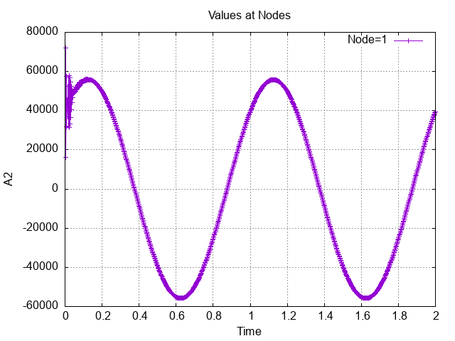
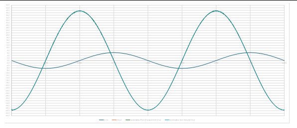
Additionally, each acceleration component should describe a sinusoidal shape with maximum amplitude 39.478 m/s2.

Each component time history of velocity against acceleration must be shifted pi/2 such that when v is max, acceleration =0 for that same component.

Then you could rotate the axis of rotation 90º to check it’s fine in other components.

You can also check other nodes (update r in formula first)

**
** Heading +++++++++++++++++++++++++++++++++++++++++++++++++
**
*Heading
Hash: mPkQWPzJ, Date: 08/08/2025, Unit system: MM_TON_S_C
**
** Nodes +++++++++++++++++++++++++++++++++++++++++++++++++++
**
*Node
1, -1.00000000E+003, -1.00000000E+003, 0.00000000E+000
2, 1.00000000E+003, -1.00000000E+003, 0.00000000E+000
3, 1.00000000E+003, 1.00000000E+003, 0.00000000E+000
4, -1.00000000E+003, 1.00000000E+003, 0.00000000E+000
5, -1.00000000E+003, -1.00000000E+003, 2.00000000E+003
6, 1.00000000E+003, -1.00000000E+003, 2.00000000E+003
7, 1.00000000E+003, 1.00000000E+003, 2.00000000E+003
8, -1.00000000E+003, 1.00000000E+003, 2.00000000E+003
9, 0.00000000E+000, -1.00000000E+003, 0.00000000E+000
10, 1.00000000E+003, 0.00000000E+000, 0.00000000E+000
11, 0.00000000E+000, 1.00000000E+003, 0.00000000E+000
12, -1.00000000E+003, 0.00000000E+000, 0.00000000E+000
13, -1.00000000E+003, -1.00000000E+003, 1.00000000E+003
14, 1.00000000E+003, -1.00000000E+003, 1.00000000E+003
15, 1.00000000E+003, 1.00000000E+003, 1.00000000E+003
16, -1.00000000E+003, 1.00000000E+003, 1.00000000E+003
17, 0.00000000E+000, -1.00000000E+003, 2.00000000E+003
18, 1.00000000E+003, 0.00000000E+000, 2.00000000E+003
19, 0.00000000E+000, 1.00000000E+003, 2.00000000E+003
20, -1.00000000E+003, 0.00000000E+000, 2.00000000E+003
21, 0.00000000E+000, 0.00000000E+000, 1.00000000E+003
22, 0.00000000E+000, 0.00000000E+000, 0.00000000E+000
**
** Elements ++++++++++++++++++++++++++++++++++++++++++++++++
**
*Element, Type=C3D20, Elset=Solid_part-1
1, 1, 2, 3, 4, 5, 6, 7, 8, 9, 10, 11, 12, 17, 18, 19,
20, 13, 14, 15, 16
**
** Node sets +++++++++++++++++++++++++++++++++++++++++++++++
**
*Nset, Nset=Node_Set-1
10
*Nset, Nset=Internal_Selection-1_Angular_Velocity-1
1, 2, 3, 4, 5, 6, 7, 8, 9, 10, 11, 12, 13, 14, 15, 16, 
17, 18, 19, 20
**
** Element sets ++++++++++++++++++++++++++++++++++++++++++++
**
*Elset, Elset=Internal_Selection-1_Solid_Section-1
Solid_part-1
**
** Surfaces ++++++++++++++++++++++++++++++++++++++++++++++++
**
**
** Physical constants ++++++++++++++++++++++++++++++++++++++
**
**
** Coordinate systems ++++++++++++++++++++++++++++++++++++++
**
**
** Materials +++++++++++++++++++++++++++++++++++++++++++++++
**
*Material, Name=S235
*Density
7.8E-09
*Elastic
210000, 0.28
*Expansion, Zero=20
1.1E-05
*Conductivity
14
*Specific heat
440000000
**
** Sections ++++++++++++++++++++++++++++++++++++++++++++++++
**
*Solid section, Elset=Internal_Selection-1_Solid_Section-1, Material=S235
**
** Pre-tension sections ++++++++++++++++++++++++++++++++++++
**
**
** Constraints +++++++++++++++++++++++++++++++++++++++++++++
**
**
** Surface interactions ++++++++++++++++++++++++++++++++++++
**
**
** Contact pairs +++++++++++++++++++++++++++++++++++++++++++
**
**
** Amplitudes ++++++++++++++++++++++++++++++++++++++++++++++
**
*Amplitude, Name=Tabular-1
0, 0, 2, 2
**
** Initial conditions ++++++++++++++++++++++++++++++++++++++
**
** Name: Angular_Velocity-1
*Initial conditions, Type=Velocity
1, 1, 6283.18530717959
1, 2, -6.28318531E+003
2, 1, 6283.18530717959
2, 2, 6283.18530717959
3, 1, -6.28318531E+003
3, 2, 6283.18530717959
4, 1, -6.28318531E+003
4, 2, -6.28318531E+003
5, 1, 6283.18530717959
5, 2, -6.28318531E+003
6, 1, 6283.18530717959
6, 2, 6283.18530717959
7, 1, -6.28318531E+003
7, 2, 6283.18530717959
8, 1, -6.28318531E+003
8, 2, -6.28318531E+003
9, 1, 6283.18530717959
10, 2, 6283.18530717959
11, 1, -6.28318531E+003
12, 2, -6.28318531E+003
13, 1, 6283.18530717959
13, 2, -6.28318531E+003
14, 1, 6283.18530717959
14, 2, 6283.18530717959
15, 1, -6.28318531E+003
15, 2, 6283.18530717959
16, 1, -6.28318531E+003
16, 2, -6.28318531E+003
17, 1, 6283.18530717959
18, 2, 6283.18530717959
19, 1, -6.28318531E+003
20, 2, -6.28318531E+003
**
** Steps +++++++++++++++++++++++++++++++++++++++++++++++++++
**
**
** Step-1 ++++++++++++++++++++++++++++++++++++++++++++++++++
**
*Step, Nlgeom, Inc=1000
*Dynamic, Solver=Pardiso
0.002, 2, 1E-05, 0.002
**
** Controls ++++++++++++++++++++++++++++++++++++++++++++++++
**
**
** Output frequency ++++++++++++++++++++++++++++++++++++++++
**
**
** Boundary conditions +++++++++++++++++++++++++++++++++++++
**
*Boundary, op=New
**
** Loads +++++++++++++++++++++++++++++++++++++++++++++++++++
**
*Cload, op=New
*Dload, op=New
**
** Defined fields ++++++++++++++++++++++++++++++++++++++++++
**
**
** History outputs +++++++++++++++++++++++++++++++++++++++++
**
*Node print, Nset=Node_Set-1, Totals=Only, Global=Yes
U, V
**
** Field outputs +++++++++++++++++++++++++++++++++++++++++++
**
*Node file
RF, U, V
*El file
S, E, ENER, NOE
**
** End step ++++++++++++++++++++++++++++++++++++++++++++++++
**
*End step
1 Like

Thank you! I’ll test it in the following days.

I’ve got some time to test it, the results: rotcube.frd

Better to work with node 10. It has a radius of 1 and it starts at zero vx=0.

This is my velocity in x history output. Looks clean and maximum amplitude as expected. 6282 mm/s.

Points of interest (zero, min, zero,max, zero,…) for velocity of node 10 are 0s, .25s, .5s,.75s,1s

Points of interest for acceleration of node 10 should be shifted (*) ..25s, .5s,.75s,1s.

(*) If velocity is a sinus, acceleration (it’s derivative) should be a cosinus.

vx component versus ax component. Node 10.

EDITED: My units are [m] sorry. I changed the titles in the graph.

Yep, sorry, I misremebered the node. I got the same diagram and A1(t=0.5) = 39474.7 mm/s2 = 39.4747 m/s2. Can we conclude that the [ACCE] output is correct (at least for this case)?

Why is so noisy around the starting point?.

It has happened the same to me when postprocessing in Excel. Velocity has probably being obtained in the same way, but as the derivative of displacements and ccx delivers a velocity that is very stable and sharp at the starting point.?¿?

If by [ACCE] you mean Ax component yes. Ac magnitude should be Ac=39.478m/s2 constant value.

Sure,

results for node 10:

  • v :check_mark:
    expected = 6.28 m/s (constant)
    simulated = 6.28 m/s (constant)
  • ac :check_mark:
    expected = 39.478 m/s^2 (constant)
    simulated = 39.492 m/s^2 (constant)
  • each acceleration component should describe a sinusoidal shape with maximum amplitude 39.478 m/s^2 :check_mark:
  • each component time history of velocity against acceleration must be shifted pi/2 such that when v is max, acceleration =0 for that same component. :check_mark:

here are the results in tabulated form:

I do not really know, I’ve used the graph command of cgx to extract the data. Maybe something is not right with my version of cgx or with the mainline ccx. I did not modify the calculation of the velocities (veold) nor the accelerations (accold), just exposed accold to frd().

I have just briefly looked through the code

Implement acceleration output

and I find a lot of places where the variable “accold” has been used, but I couldn’t find any single place where variable “accold” has been declared. Please remember, a proto type declaration in C doesn’t count for an allocation for the variable.

Off course I could be wrong, but in case my assumption is correct, that could be a possible reason for all the noise in the beginning of the curves.

I’ve tried different solvers, but this noise is odd. It is consinstent, so it is not an uninitialised variable. I’ll try to look into it.


I’ve run the pendel example:

**
**   Structure: pendulum.
**   Test objective: dynamic calculation with large rotations.
**
*NODE,NSET=NALL
1, 0.0, 0.0, 0.0
2, 0.0, 0.0, -15.0
3, 0.0, 0.0, -30.0
4, 0.0, 0.0, -30.0
5, 0.0, 0.0, -180.0
6, 0.0, 0.0, -330.0
*ELEMENT, TYPE=B32, ELSET=ELALL
1, 1,2,3
2, 4,5,6
*BEAM SECTION, MATERIAL=STEEL, ELSET=ELALL, SECTION=RECTANGULAR
10,10
0.0, 1.0, 0.0
*EQUATION
2, 
3, 1, -1.0, 4, 1, 1.0
2,
3, 3, -1.0, 4, 3, 1.0
**
** EBENE BEWEGUNG IN (X,Z)
*BOUNDARY
NALL, 2,2
NALL, 4,4
NALL, 6,6
1, 1,3
*MATERIAL, NAME=STEEL
*ELASTIC
200000.0, 0.3
*DENSITY
7.8E-09, 
*INITIAL CONDITIONS, TYPE=DISPLACEMENT
NALL, 1, 0.0
NALL, 3, 0.0
*INITIAL CONDITIONS, TYPE=VELOCITY
NALL, 1, 0.0
NALL, 3, 0.0
*NSET,NSET=N1
6
**
** IN 1000 SEC 1000 MAL DREHEN
*AMPLITUDE, NAME=RAMP
0.0, 0.0, 1000.0, 6280.0 
*STEP, NLGEOM, INC=1000000
*DYNAMIC, ALPHA=-0.30
0.00001, 1.0, 0.000000001
*BOUNDARY, AMPLITUDE=RAMP
1, 5,5, 1.000
*DLOAD
ELALL, GRAV, 9810.0, 0.0, 0.0, -1.0
*NODEFILE
U,V,A
*END STEP

and got the “noise” in the accelerations:


Looks like the initial value of the acceleration is somewhat wrong.

Both rotcube and pendel has the output:

 *INFO reading *STEP: nonlinear geometric
       effects are turned on

and use the calculations from nonlingeo.c.

Acceleration noise comes from the derivation scheme.

I have use the direct solver to have a constant time step of 0.002 (this way errors coming from discrepancy in the time increment disappear)

I have applied a Forward Finite-Difference for the first two point O(h2).

I have applied a Centered Finite-Difference for intermediate points O(h4).

I have applied a Backward Finite-Difference for the Last two point O(h2).

I have computed acceleration directly from displacements.

Noise has disappeared.

I don’t have skills to dive into the ccx code to find the derivation scheme for velocity but It could be interesting to find how it’s done.Specially for the first points when time increment in not regular.

1 Like

When time increments are not regular, (specially at the starting point or areas in which the convergence is struggling and time increment is reduced) the derivative of the time history is not so direct. As you have more than two terms involved for higher order aproximations, there is not a unique “h”. Other methos are required. I guess if Don Guido is using polynomial approximation for those points.

Thank you! My primary goal was to output the accelerations to the .frd file, and I think it was achieved with your help. The output showed that the calculation of the acceleration can be improved, but that is a different problem.

I’ve just started to get familiar with the codebase, so I cannot say that I can solve this, but I’ll try to take a look. Your insight is a very good starting point. I’ll do a PR if I find something.

many thanx for your work.

It seems is a usual problem especially in highly nonlinear dynamic problems: https://asmedigitalcollection.asme.org/IMECE/proceedings-abstract/IMECE2000/19333/67/1126113

Not sure if this example fits that typology.

1 Like