I am a newbie in vibration modeling, so apologies in advance if this is an ill-posed question. I seem to be running into a peculiar output from CalculiX, and wondering if anyone has any insights into it.
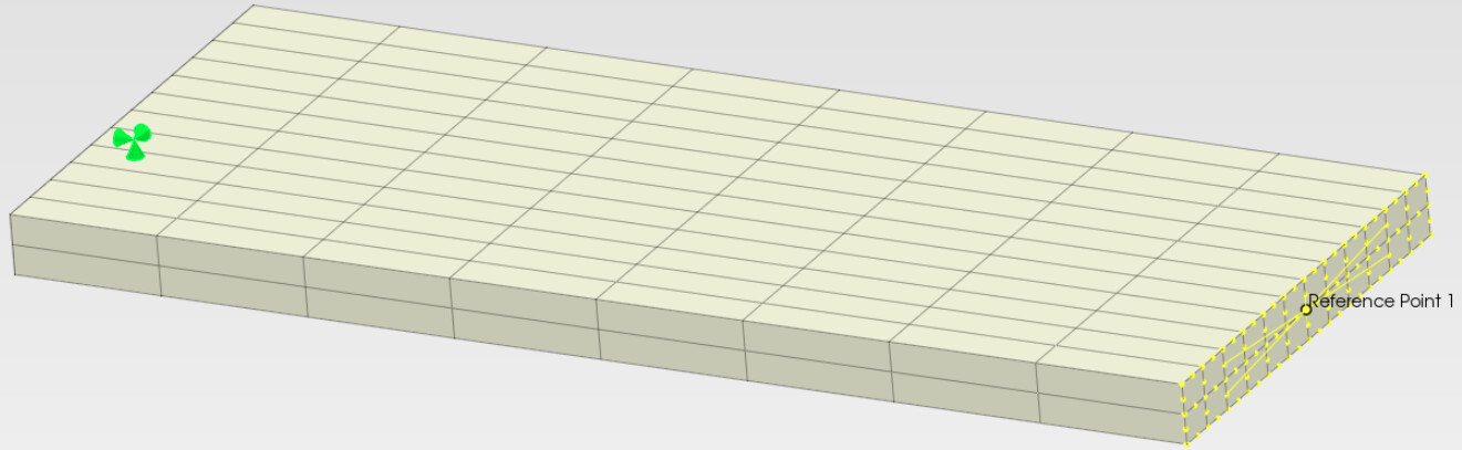
To better understand the general 3D modeling capability, I wanted to solve a harmonic analysis for a beam with a point mass at the tip, loaded at the base by *base motion. Below is the picture of the model. One end is fixed by a homogeneous *boundary, while the other end has a point mass at the reference point, which is connected to the set of end nodes.
I first ran the *frequency step to solve for a few natural frequencies, then ran the *steady state dynamics step with *base motion applied in y-direction of the homogeneous boundary.
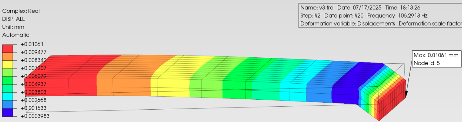
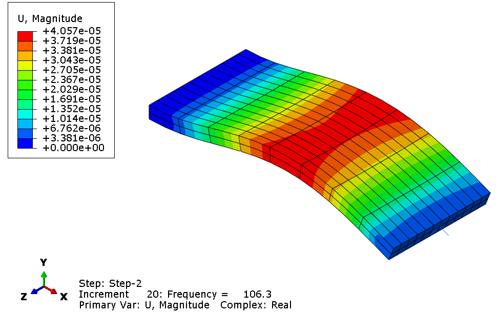
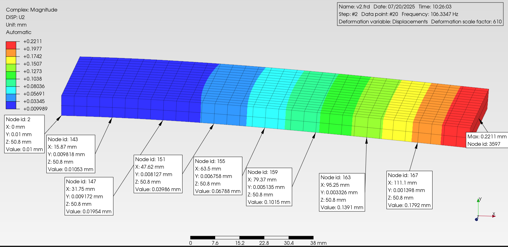
The displacement results below appear to show a kink in the tip elements of the beam. The plot is for real displacement, but even the magnitude has the same trend. I am a bit puzzled by such a kink happening abruptly at the tip.
If I use the force load instead of base motion, the outputs look reasonably good; so this appears to be happening with the base motion only. I wonder if this has something to do with the point mass I am using at the tip? Could there be some incompatibility issue here between the point mass and the base motion?
I have the full model set-up below if anyone would like to look into it:
Ideally, start simpler… No point mass at the tip. Understand the capabilities and limitations with a simple beam of known solutions.
You need to request more modes in order for them to be active during your steady-state dynamics analysis… If you only request 3 modes, then your steady-state will only have access to those extracted modes. → Abaqus mentions: “In a mode-based steady-state dynamic analysis the response is based on modal superposition techniques; the modes of the system must first be extracted using the eigenfrequency extraction procedure. The modes will include eigenmodes and, if activated in the eigenfrequency extraction step, residual modes. The number of modes extracted must be sufficient to model the dynamic response of the system adequately, which is a matter of judgment on your part.”
You may want to split those elements longitudinally at least in half to avoid any ill-shaped elements. As for the physics behind the kink, isn’t your point mass a few times heavier than the beam itself?? Maybe my calculation was off…
Thanks a lot JBR for your feedback. I tried the following after your suggestions:
Added 30 modes to the frequency step, the solution didn’t change, probably the mass at the tip is dominating in terms of the first rocking mode
Refined the mesh to 4x more elements along the length, tip kinking is still there. Interestingly, it is the last (tip) elements that undergo such kinking only. This makes me think the point mass along with the rigid body constraints to it might be the culprit here when the *base motion is used.
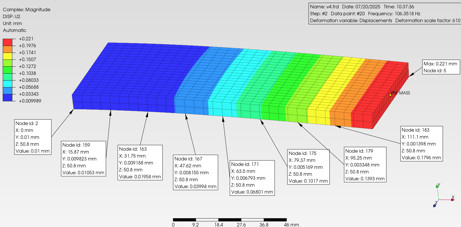
Eliminated the point mass and connections, and instead I set the last layer of elements to be denser (heavier), simulating the tip mass. This solution didn’t have any issues with kinking.
It looks like the *base motion boundary option does not support the point mass, but I didn’t find a statement in the manual, so I am not sure. It would be nice to know if anyone else had such an issue.
I can’t think of any physics issue here. Even if the beam had relatively insignificant mass, this problem could be approximated as a single DOF spring-mass system. Then, whether you apply the forcing function or base excitation, you would expect the same outcome, isn’t it? What is puzzling is that kinking is present only with the base motion, not with the cload. On top of that, the kinking is always present in the last element, no matter what the length of that element is, which seems more like a non-physics-related issue. But if you have anything specific in mind, please let me know, I am curious.
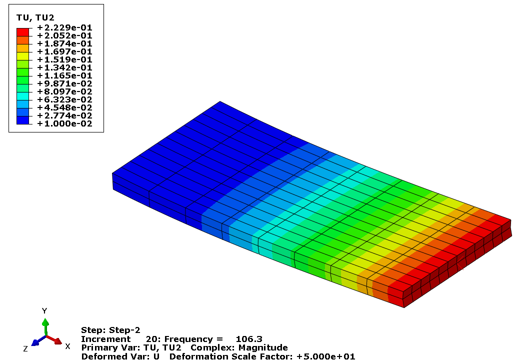
Thanks a lot for sharing the Abaqus results. It is interesting to see no kinking is present in Abaqus solution. I am wondering if this solution is for the TYPE=ACCELERATION (default) or DISPLACEMENT? The reason why I ask is because I was expecting the displacement output in the contour plot to be the input amplitude (0.01 mm) at the base.
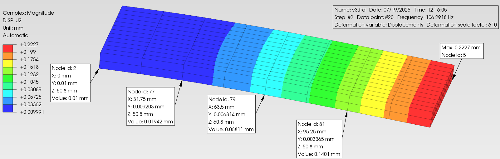
In calculiX there seems to be a way around for base displacement input. If I apply the base displacement excitation via the non-zero *boundary keyword instead of *base motion, it seems like I am getting a more realistic solution as shown below. You see, in this solution, the base displacement is the input displacement, while the tip displacement is amplified because of the dynamic effect at this freq (close to the natural freq). It would be nice to cross-check this solution with Abaqus.
I am still not sure about the *base motion approach with the point mass, but I can try the distributed mass option as you suggested and post my findings here. If it can be confirmed that the point mass issue is a bug, we may want to submit a bug report for it, but there’s a chance I may not be implementing it correctly in the input file I released in my original post.
I only changed the keywords that had to be changed to run it in Abaqus. Otherwise, it was the same input deck so the *BASE MOTION keyword remained unchanged as well.
CalculiX allows this approach but Abaqus doesn’t:
It is not possible to prescribe nonzero displacements and rotations directly as boundary conditions in mode-based dynamic response procedures. Therefore, in a mode-based steady-state dynamic analysis, the motion of nodes can be specified only as base motion; nonzero displacement or acceleration history definitions given as boundary conditions are ignored, and any changes in the support conditions from the eigenfrequency extraction step are flagged as errors.
Unfortunately, I do not have Abaqus experience to tell what is happening there, but I still have doubts about the Abaqus results. It doesn’t seem to be solving the problem as defined, because I would think the base displacement would at least be the same as the input displacement amplitude, which is 0.01 mm. Perhaps, I am not interpreting the results correctly.
On the other hand, I tried to use the distributed mass option as you suggested, along with the *base motion loading. The results came out to be very similar to the *boundary option as shown below. I have two main conclusions from this:
The non-zero *boundary loading at the base could be a workaround for base displacement when the point mass is used. This option does not allow direct base acceleration input, but the displacement input should be adequate to generate transmissibility output for the model. Alternatively, the distributed mass can be used with the *base motion. Luckily Prepomax makes the job easy to distribute the mass if this option is used.
From what I understand, the main difference between the point-mass and the distributed mass is the rigid body constraints. So I am suspecting the rigid body constraints are causing the inaccurate displacements and kinking issues in the *base motion based analyses.
Thank you for suggesting to try the distributed mass option.
I just learned that abaqus by default outputs the relative displacements. So the contour you provided is potentially for the relative displacements, while calculix outputs the total displacements. It is based on this extract from abaqus manual:
The standard output variables U, V, A, and the variable PU listed above correspond to motions relative to the motion of the primary base in a mode-based analysis. Total values, which include the motion of the primary base, are also available:
TU - Magnitude of all components of total displacement/rotation at a node.
There doesn’t seem to be an easy way for me to process calculix output to convert it to relative displacement, but per the manual extract above, one can use TU in abaqus to export the total displacements. If you happen to have the model handy, it would be nice if you can try to drop the TU contour plot here. Just curious if the displacement solutions match.
Thanks a lot for posting this result. The contour plot looks encouragingly similar to the calculiX results that I posted up above using the workaround analysis methods.
I submitted a bug report regarding this issue. Hopefully it will get resolved at some point.