right, someone need to consider warping support conditions were classical formulation ignoring this.
using *RIGID BODY with the entire cross-section and translation at the supports
in length direction is fixed is like fixed warping displacement.
why is there no change of the result if i fix only one support in length direction?
in LTBEAM the result is different, but ccx it has no influence!?
also with *DISTRIBUTING!?
because both supports are fixed in cross / traverse direction.
so with RIGID BODY and entire cross-section warping displacement is fixed,
with *DISTRIBUTING warping displacement is free.
solution is with *RIGIG BODY to create two support over the cross-section,
one for the upper part one for the lower part,
or fixing only the web, or better, create the web with thickness 2 elements and
fix only the nodes in the middle and in the web.
to be continued
Hi dichtstoff,
I have read in the ReleaseInfo.txt file contained in the LTB folder this:
Version N°1.0.6 Release date: 07/2005
Fixed errors:
. correction in units of restraining springs for teta (torsion) and teta’ (warping) (“/rd” added)
That would suggest some springs are probably used to properly constrain the beam and help to make warping effect to emerge.
It should also be more noticeable in short beams.
I’m looking for the proper way to apply BC for warping to show up.
EDITED: Found this in the help.

Hello Disla,
i have fixed for *RIGID BODY only the nodes from web,
and the results are adorable:
**** centric pressure: 1.000,0
**** lateral buckling: 4.385,0 ccx: 4.405,0 0,005 %
**** lateral buckling: 15.877,0 ccx: 15.242,0 0.040 %
**** torsional buckling: 10.427,0 ccx: 11.233,0 0.077 %
**** bending moment: 1.000.000,0
**** lateral torsional buckling: 1.502,0 ccx: 1.534,0 0,021 %
if fix the entire cross-section at support,
what triggers the fixed warp displacement?
wbr


Hi,
I have downloaded your files. Unfortunately, there was no msh file to identify where those BC were applied.
I have also seen you use solids (SOLID SECTION) and nonlinear geometric analysis (*** proof of lateral buckling by nonlinear geometric calculation).
¿I’m I right.? ¿How many nodes are involved to get that accuracy?
None of the coupling cards works for me with shells.
Regards
¿How do you compute the deviation?¿Is doesn’t seems percentage %?
*** lateral buckling: 4.385,0 ccx: 4.405,0 (4.385,0-4.405,0)/4.385,0*100 = 0.45%
Hi,
i have upload all files.
i have forgotten the 100 in calc.
i have also upload the shell-beam example
wbr dichtstoff
In fact for thick profiles warping isn’t relevant most of the time.
Is NLGEOM activated? buckling is a linear procedure so it doesn’t activates non linear effects by default.
Hi,
I’m working on the IP 448x400x24x12.
The beam technique as support on the extreme wedges has shown to perform pretty well on shells without the need of Distributing.
I would like to finish the analysis for comparison, but I don’t have clear what does it mean the BC called
**** bending moment 1.000.000 / **** lateral torsional buckling: 1.502,0
****BENDING MOMENT
Nrotnode_01,2, 1000000
Nrotnode_02,2,-1000000
****BENDING MOMENT
¿Are these opposite moments of +/- 1 KN/m on each extreme of the beam?
Thanks

yes, unit load with 1.0 kN x 1000 N 1.0 m x 1000 mm
do you know how you can place here a text with scrollbar?
wbr
Click the “Preformatted text” option (or press Ctrl+E).
This is my results.
Buckling factor in the strong axis differs the most in a 4% .
Apart from the FEA result I have serious doubts the Euler’s formula used in STALBAU III as a reference has applicability for this beam.
This section (l/k) ratio for the strong axis is too low for the Euler formula applicability.
I’m using a beam element as said in the LTBeam Validation on each side (only web) and it works well.
There is no need to use *DISTRIBUTING or Rigid Body. Loads and BC are applied directly to that beams. That fact allows me to use ccx v2.19 and shells.


this may caused by offset in the model, another possibility are support modeling.
below figures & tables i have got in 2015 for case of distributed loads,


stiff beam approach is similar to MPC or Rigid Body itself, this is not recommended since it may lead to numerical problems or conflict with another features (e.g contact, plasticity) but still can be use with cautions.
I have changed my system with solid elements,
i fixed one end and applied 1000 N on the other end.
fixed and load on nodes directly:
*BOUNDARY
Nsbound_01,1,3,0
*CLOAD
Nsbound_02,3,-18.51852
total force (fx,fy,fz) for set NSBOUND_01 and time 0.0000000E+00
2.684040E-10 2.313234E-10 1.000000E+03
total force (fx,fy,fz) for set NSBOUND_02 and time 0.0000000E+00
-5.163383E-12 -3.188363E-12 -1.000000E+03
lateral buckling weak axis: (1096-1107)/1096100 = 1,00 %
lateral buckling strong axis: (3969-3944)/3969100 = 0.63 %


Hi dichtstoff,
I have scaled my beam to measure twice the actual length .¿ Same as you ?.
Lateral buckling weak axis: (1096-1096)/1096 x 100 = 0,00 % deviation
Lateral buckling strong axis: (3969-3932)/3969 x 100 = 0.93 % deviation.
The mixture of shells with small beams to help support works nice. I will use it with caution untill *RIGID BODY and DISTRIBUTING are available for shells.
I would say that the deviations seen with the Stahlbau III pag 29 is because Euler’s formula is not appropriate for the beam used in the example. Slender ratio is too small.
Johnson’s parabolic would be a safety option if one wants a theoretical reference.
1 Like
Hi Disla,
thnx a lot. I’ll check these Johnson’s parabolic.
Can you calc. by hand the values for buckling strong axis with johnson’s parabolic?
or what is the criteria between euler and johnson?
I take so much out with these discussion.
I know how to handle now the support for lateral torsional buckling.
Anyway, I still prefer to work with solid elements,
I’ll try to update my example.
thnx to all, I’m so happy. ![]()
wbr dichtstoff
You have some notes of Johnson’s parabolic in Wikipedia with a reference for the validity range of Euler’s formula.
Strong axis (l/k) is about half below the critical value. If a column has (l/k)<(l/k)cr you must pay attention to other failure mechanisms as it may reach the plastic range before buckling. Nonlinear buckling analisys with plasticity would be required.
| Strong Axis | Weak Axis | ||||
|---|---|---|---|---|---|
| Pcr | 15.877,27 | KN | 4.385,04 | KN | |
| (l/k) | 56,0 | 106,5 | |||
| (l/k)cr | 108,1 | 108,1 |
Hello Disla,
I’m not convinced with your thesis about Johnson’s parabolic,
because it is empirically based equation.
what have you in mind, when you say nonlinear buckling analysis?
wbr
Johnson’s parabolic considers that some beam geometries overpass the yield point way before the Ncr is reached.
If your first buckling mode would have been Ncr=15.877 KN , by that time, you would have 661 Mpa in the section.
Nonlinear buckling, I mean to introduce some geometric imperfections ( better with plasticity here ) and run an increasing load/displacement up to the point where the buckling shape starts to show.
If you want to see the aftermath of reaching 15.877KN you would need to adjust BC to remove the first two modes and make Ncr3 to become Ncr1.See pict.

Hello Disla,
maybe we should open a new topics.
the reason for the discrepancy is not yet defined or spotted for me.
you connect these with Johnson’s parabolic where you have a yield point,
but we don’t use or have these in eigenvalue Buckling Analysis.
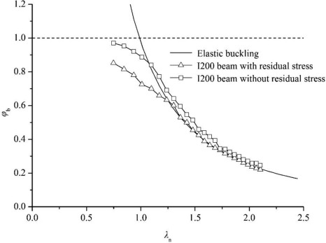
If you show me how to apply residual stress for these profile,
i start immediately with nonlinear buckling ![]()